GIS Shortcuts

Miscellaneous gis notes, mostly derived from my blog over here
Index:
eBird API stuff
R / Shiny Web Experiments
Shell macros from R
When it must be Windows
Windows WSL - Ubuntu GDAL setup
Ubuntu & Jupyter cartopy setup
Mac OSX - GDAL setup
Bash Example - DEM stitching
Link to rJDK management info
eBird regionCode
The Ebird dataset is awesome. While directly handling data as a massive delimited file- as distributed by the eBird people- is cumbersome at best, the ebird api offers a fairly straightforward and efficient alternative for a few choice bits and batches of data.
-
The eBird
AWKtool for filtering the actual delimited data can be found over here:install.packages("auk")
It is worth noting R + auk (or frankly any R centered filtering method) will quickly become limited by the single-threaded approach of R, and how you’re managing memory as you iterate. Working and querying the data from a proper database quickly becomes necessary.
Most conveniently, the eBird API already exists.
…The API package for R is over here:
...There is also a neat Python wrapper [over here](https://pypi.org/project/ebird-api/):
```pip3 install ebird-api```

***Region Codes:***

I'm not sure why, but some methods use normal latitude / longitude in decimal degrees while some others use `"regionCode"`, which seems to be some kind of eBird special.  Only ever seen this format in ebird data.

For example, recent observations uses `regionCode`:
```shell script
# GET Recent observations in a region:
# https://api.ebird.org/v2/data/obs//recent
…But nearby recent observations uses latitude / longitude:
# GET Recent nearby observations:
# https://api.ebird.org/v2/data/obs/geo/recent?lat=&lng=
Regardless, lets just write a function to convert decimal degrees to this regionCode thing. Here’s mine:
#!/usr/bin/env python3
"""
# provide latitude & longitude, return eBird "regionCode"
Written by Jess Sullivan
@ https://transscendsurvival.org/
"""
import requests
import json


def get_regioncode(lat, lon):

    # this municipal api is a publicly available, no keys needed afaict
    census_url = str('https://geo.fcc.gov/api/census/area?lat=' +
                     str(lat) +
                     '&lon=' +
                     str(lon) +
                     '&format=json')

    # send out a GET request:
    payload = {}
    get = requests.request("GET", census_url, data=payload)

    # parse the response, all api values are contained in list 'results':
    response = json.loads(get.content)['results'][0]

    # use the last three digits from the in-state fips code as the "subnational 2" identifier:
    fips = response['county_fips']

    # assemble and return the "subnational type 2" code:
    regioncode = 'US-' + response['state_code'] + '-' + fips[2] + fips[3] + fips[4]
    print('formed region code: ' + regioncode)
    return regioncode
GIS Wigdets, Web Apps & R/ Shiny
Some experiments with simple web utilities for GIS tasks.
Process manager experiments for R threads in /Flask-Manager.
Visit the single threaded example here; (Not load balanced, just for an example view). These are wrapped in a Node.JS application on Heroku, which loads each utility through shinyapps.io. These functions are hosted entirely through (Heroku / shinyapps) free tiers.
See /Docker-App for deployment in the GCP app engine.
- Raster2stl - converts raster data (image- a .jpg taken from a DEM file for instance) to a 3d STL file showing exagerated terrain. (added 3/6/19)
- KML2SHP_Converter - generates a zip archive of shape files based on KML file layers
- Centroid_KML - “KML-Centroid-Generator”
- KML2CSV - converts KML (XML) to .csv spreadsheet format
- KMLSubsetFilter - from a KML file, this tool returns a subset KML based on two query strings (searches the description field of the KML)
Some more Bits, Bobs, Widgets & R / Shiny demos:
|  |
|  |
|—|—|
|
|—|—|
Some GDAL shell macros from R instead of rgdal
it’s not R sacrilege if nobody knows
Even the little stuff benefits from some organizational scripting, even if it’s just to catalog one’s actions. Here are some examples for common tasks.
Get all the source data into a R-friendly format like csv. ogr2ogr has a nifty option -lco GEOMETRY=AS_WKT (Well-Known-Text) to keep track of spatial data throughout abstractions- we can add the WKT as a cell until it is time to write the data out again.
# define a shapefile conversion to csv from system's shell:
sys_SHP2CSV <- function(shp) {
  csvfile <- paste0(shp, '.csv')
  shpfile <-paste0(shp, '.shp')
  if (!file.exists(csvfile)) {
    # use -lco GEOMETRY to maintain location
    # for reference, shp --> geojson would look like:
    # system('ogr2ogr -f geojson output.geojson input.shp')
    # keeps geometry as WKT:
    cmd <- paste('ogr2ogr -f CSV', csvfile, shpfile, '-lco GEOMETRY=AS_WKT')
    system(cmd)  # executes command
  } else {
    print(paste('output file already exists, please delete', csvfile, 'before converting again'))
  }
  return(csvfile)
}
Read the new csv into R:
# for file 'foo.shp':
foo_raw <- read.csv(sys_SHP2CSV(shp='foo'), sep = ',')
One might do any number of things now, some here lets snag some columns and rename them:
# rename the subset of data "foo" we want in a data.frame:
foo <- data.frame(foo_raw[1:5])
colnames(foo) <- c('bar', 'eggs', 'ham', 'hello', 'world')
We could do some more careful parsing too, here a semicolon in cell strings can be converted to a comma:
# replace ` ; ` to ` , ` in col "bar":
foo$bar <- gsub(pattern=";", replacement=",", foo$bar)
Do whatever you do for an output directory:
# make a output file directory if you're into that
# my preference is to only keep one set of output files per run
# here, we'd reset the directory before adding any new output files
redir <- function(outdir) {
  if (dir.exists(outdir)) {
    system(paste('rm -rf', outdir))
  }
  dir.create(outdir)
}
Of course, once your data is in R there are countless “R things” one could do…
# iterate to fill empty cells with preceding values
for (i in 1:length(foo[,1])) {
  if (nchar(foo$bar[i]) < 1) {
    foo$bar[i] <- foo$bar[i-1]
  }
  # fill incomplete rows with NA values:
  if (nchar(foo$bar[i]) < 1) {
    foo[i,] <- NA
  }
}

# remove NA rows if there is nothing better to do:
newfoo <- na.omit(foo)
Even though this is totally adding a level of complexity to what could be a single ogr2ogr command, I’ve decided it is still worth it- I’d definitely rather keep track of everything I do over forget what I did…. xD
# make some methods to write out various kinds of files via gdal:
to_GEO <- function(target) {
  print(paste('converting', target, 'to geojson .... '))
  system(paste('ogr2ogr -f', " geojson ",  paste0(target, '.geojson'), paste0(target, '.csv')))
}

to_SHP <- function(target) {
  print(paste('converting ', target, ' to ESRI Shapefile .... '))
  system(paste('ogr2ogr -f', " 'ESRI Shapefile' ",  paste0(target, '.shp'), paste0(target, '.csv')))
}

# name files:
foo_name <- 'output_foo'

# for table data 'foo', first:
write.csv(foo, paste0(foo_name, '.csv'))

# convert with the above csv:
to_SHP(foo_name)
Using Ubuntu GDAL on Windows w/ WSL
LINK: get the WSL shell from Microsoft
# In the WSL shell:

sudo apt-get install python3.6-dev -y
sudo add-apt-repository ppa:ubuntugis/ppa && sudo apt-get update
sudo apt-get install libgdal-dev -y
sudo apt-get install gdal-bin -y

# See here for more notes including Python bindings:
# https://mothergeo-py.readthedocs.io/en/latest/development/how-to/gdal-ubuntu-pkg.html
In a new Shell:
# Double check the shell does indeed have GDAL in $PATH:
gdalinfo --version
Ubuntu & Jupyter: cartopy setup
# install libraries:
sudo apt install libproj-dev proj-data proj-bin
sudo apt install libgeos-dev
# install cython, cartopy:
pip3 install cython
pip3 install cartopy
# fix shapely:
pip3 uninstall shapely
pip3 install shapely --no-binary shapely
Using GDAL on Mac OSX
Note: in my opinion, homebrew and macPorts are good ideas- try them! If you don’t have Homebrew, get it now:
/usr/bin/ruby -e "$(curl -fsSL https://raw.githubusercontent.com/Homebrew/install/master/install)"
(….However, port or brew installing QGIS and GDAL (primarily surrounding the delicate links between QGIS / GDAL / Python 2 & 3 / OSX local paths) can cause baffling issues. If possible, don’t do that. Use QGIS installers from the official site or build from source!)
if you need to resolve issues with your GDAL packages via removal: on MacPorts, try similar:
sudo port uninstall qgis py37-gdal

# on homebrew, list then remove (follow its instructions):

brew list
brew uninstall gdal geos gdal2
!!! NOTE: I am investigating more reliable built-from-source solutions for gdal on mac.
Really!
There are numerous issues with brew-installed gdal. Those I have run into include:
- linking issues with the crucial directory “gdal-data” (libraries)
- linking issues Python bindings and python 2 vs. 3 getting confused
- internal raster library conflicts against the gdal requirements
- Proj.4 inconsistencies (see source notes below)
- OSX Framework conflicts with source / brew / port (http://www.kyngchaos.com/software/frameworks/)
- Linking conflicts with old, qgis default / LTR libraries against new ones
- Major KML discrepancies: expat standard vs libkml.
brew install gdal
#
# brew install qgis can work well too.  At least you can unbrew it!
#
Next, assuming your GDAL is not broken (on Mac OS this is rare and considered a miracle):
# double check CLI is working:
gdalinfo --version
# “GDAL 2.4.0, released 2018/12/14”
gdal_merge.py
# list of args
Regarding Windows-specific software, such as ArcMap
Remote Desktop:
The greatest solution I’ve settled on for ArcMap use continues to be Chrome Remote Desktop, coupled with an IT Surplus desktop purchased for ~$50. Once Chrome is good to go on the remote Windows computer, one can operate everything from a web browser from anywhere else (even reboot and share files to and from the remote computer). While adding an additional, dedicated computer like this may not be possible for many students, it is certainly the simplest and most dependable solution.
VirtualBox, Bootcamp, etc:
Oracle’s VirtualBox is a longstanding (and free!) virtualization software. A Windows virtual machine is vastly preferable over Bootcamp or further partition tomfoolery.
One can start / stop the VM only when its needed, store it on a usb stick, avoid insane pmbr issues, etc.
- Bootcamp will consume at least 40gb of space at all times before even attempting to function, whereas even a fully configured Windows VirtualBox VDI will only consume ~22gb, and can be moved elsewhere if not in use.
- There are better (not free) virtualization tools such as Parallels, though any way you slice it a dedicated machine will almost always be a better solution.
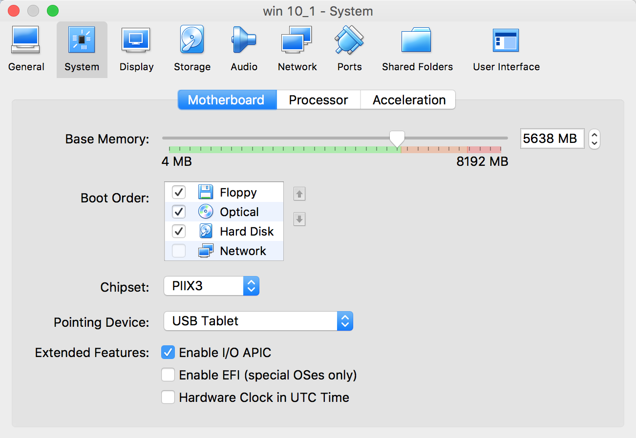
Setup & Configure VirtualBox:
There are numerous sites with VirtualBox guides, so I will not go into detail here.
Extra bits on setup-
- Guest Additions are not necessary, despite what some folks may suggest.
- Dynamically Allocated VDI is the way to go as a virtual disk. There is no reason not to set the allocated disk size to the biggest value allowed, as it will never consume any more space than the virtual machine actually needs.
-
Best to click through all the other machine settings just to see what is available, it is easy enough to make changes over time.
- There are many more levels of convoluted not worth stooping to, ranging from ArcMap via AWS EC2 or openstack to KVM/QEMU to WINE. Take it from me
Using ESRI ArcGIS / ArcMap on Macs, continued…
I need to run ESRI products on my MacBook Pro. QGIS is always the prefered solution- open source, excellent free plugins, works on mac natively- but in a college / research environment, the only option that supports other people and school machines is ESRI. Despite the annoying bureaucracy and expense of the software, some things are faster (but not better!) in ESRI, like dealing with raster / multiband data.
First, you need a license.
I went about this two ways;
My first solution was to buy an ESRI Press textbook on amazon. A 180 day trial for $50- when taken as a college course, this isn’t to bad. :) The book is slow and recursive, but a 180 days to play with all the plugins and whistles allows for way deeper learning via the internet. :)
Do know there is a little-documented limit to the number of license transfers you may perform before getting either lock in or out of your software. I hit this limit, as I was also figuring out my virtual machine situation, which would occasionally need a re-installation.
My current solution is “just buy a student license”. $100 per year is less than any adobe situation- so really not that bad.
Now you need a windows ISO.
https://www.microsoft.com/en-us/software-download/windows10ISO
Follow that link for the window 10, 64 bit ISO. YOU DO NOT NEED TO BUY WINDOWS. It will sometimes complain about not having an authentication, but in the months of using windows via VMs, never have I been prohibited to do… anything. When prompted for a license when configuring your VM, click the button that says “I don’t have a license”. Done.
Option one: VirtualBox VM on a thumbdrive
https://www.virtualbox.org/wiki/Downloads - VirtualBox downloads- the VM will take up most of a 128gb flash drive- ~70 gb just for windows and all the stuff you’ll want from a PC. Add ESRI software and allocated space for a cache (where your GIS project works!), bigger is better. Format all drives in disk utility as ExFat! this is important, any other file system either won’t fly or could wreak havoc (other FAT based ones may have too small file allocations!
I used two drives, a 128 and a 64- this is great because I can store all my work on the 64, so I can easily plug it into other (school) machines running windows ArcMap and keep going, without causing issues with the massive VM in the 128.
Installation is straightforward- added more screenshots of the process in vmsetup
Problems: Stability. Crashes, and python / some other script modules do not work well. This is a problem. ArcAdministrator gets confused about all kinds of things- FWIW, if you are googling to delete the FLEXnet folder to solve authentication file issues, move to option 2 :)
Speed is down, but actually the ~same speed as our school “super” PCs- (though I happened to know they are essentially glorified “hybrid” VMs too!) .

Option two: OSX Bootcamp
https://support.apple.com/boot-camp
https://support.apple.com/en-us/HT201468
This way, you will hit “option/alt” each time you restart/boot your computer to choose from win/osx. This is easy to install, as it is mac and mac = easy.
Big Caveat: it is much harder to install windows externally (on a usb, etc) from bootcamp. I didn’t succeed in my efforts, but there could be a way…. The thing is, it really wants to run everything like a normal intel based PC, with all installations in the usual place. This is good for the mac performance, but terrible for the tiny SSD hard drives we get as mac users. I have a 256gb SSD. I have an average of < 15 gb wiggle room here, and use every cloud service in the book.
If you need to manage your cloud storage because of a itsy mac SSD, my solution is still ODrive. https://www.odrive.com/
Example DEM stiching from GDAL
To begin- try a recent GIS assignment that would otherwise rely on the ESRI mosaic system:
Data source: ftp://ftp.granit.sr.unh.edu/pub/GRANIT_Data/Vector_Data/Elevation_and_Derived_Products/d-elevationdem/d-10m/
# wget is great, and is included in many distributions- it is not installed by default on Mac OSX however.

brew install wget
make some folders
mkdir GIS_Projects && cd GIS_Projects
use wget to download every .dem file (-A .dem) from the specified folder and sub-folders (-r)
wget -r -A .dem ftp://ftp.granit.sr.unh.edu/pub/GRANIT_Data/Vector_Data/Elevation_and_Derived_Products/d-elevationdem/

cd ftp.granit.sr.unh.edu/pub/GRANIT_Data/Vector_Data/Elevation_and_Derived_Products/d-elevationdem
make an index file of only .dem files.
(If we needed to download other files and keep them from our wget (more common)
this way we can still sort the various files for .dem)
ls -1 *.dem > dem_list.txt
use gdal to make state-plane referenced “Output_merged.tif” from the list of files in the index we made. We will use a single generic “0 0 255” band to show gradient.
gdal_merge.py -init "0 0 255" -o Output_Merged.tif --optfile dem_list.txt
copy the resulting file to desktop, then return home
cp Output_Merged.tif ~/desktop && cd
if you want (recommended):
rm -rf GIS_Projects # remove .dem files. Some are huge!
In Finder at in ~/desktop, open the new file with QGIS. A normal photo viewer will NOT show any detail.
Need to make something like this a reusable script? In Terminal, just a few extra steps:
mkdir GIS_Scripts && cd GIS_Scripts
open an editor + filename. Nano is generally pre-installed on OSX.
nano GDAL_LiveMerge.sh
COPY + PASTE THE SCRIPT FROM ABOVE INTO THE WINDOW
- ctrl+X , then Y for yes
make your file runnable:
chmod u+x GDAL_LiveMerge.sh
run with ./
./GDAL_LiveMerge.sh
You can now copy + paste your script anywhere you want and run it there. scripts like this should not be exported to your global path / bashrc and will only work if they are in the directory you are calling them: If you need a global script, there are plenty of ways to do that too.
See /Notes_GDAL/README.md for notes on building GDAL from source on OSX
